ON SEA LEVEL ALONG THE BRAZILIAN COAST - PART II

Afrânio Rubens de Mesquita- Departamento de Oceanografia Física, Instituto Oceanográfico-USP, Praça do Oceanográfico, 191 CEP: 05508-900 Cidade Universitária, São Paulo, Brasil ardmesqu@usp.br

Alberto dos Santos Franco- Departamento de Oceanografia Física, Instituto Oceanográfico-USP, Praça do Oceanográfico, 191 CEP: 05508-900 Cidade Universitária, São Paulo, Brasil) asfranco@intercall.com.br

Joseph Harari- Departamento de Oceanografia Física, Instituto Oceanográfico-USP, Praça do Oceanográfico, 191 CEP: 05508-900 Cidade Universitária, São Paulo, Brasil) joharari@usp.br

Carlos Augusto de Sampaio França(Departamento de Oceanografia Física, Instituto Oceanográfico-USP, Praça do Oceanográfico, 191 CEP: 05508-900 Cidade Universitária, São Paulo, Brasil) cafranca@usp.br

ABSTRACT

This is Part II of a contribution on Brazilian sea levels - Part I dealt with the seasonal variability -. It examines the sea level changes along the Brazilian coast from series with less than 40 years of measurement, against the background of changes in series of all continents and islands around the world, considering data distributed by the Permanent Service for Mean Sea Level (PSMSL). The description follows the display of the data in a first plot of relative sea level trends (C), against the length of the series (L) in years and a second plot showing relative sea level trends (C), against the correlation values (m), of the data of each series and the data of its regression line. The first plot of all PSMSL data exhibited a cuspid like shape of the distribution of (C), having maxima values about 10-20 cm/cty for the longest series (120-137 years). Similar plot of African and South American data adjusted to the same relative mean level, showed that the Brazilian trends (C), are mostly concentrated in the positive side of the cuspid (ports of Belem, Fortaleza. Recife, Canavieiras, Salvador, Ilha Fiscal, Rio de Janeiro, Ubatuba, Cananéia, and Imbituba). Salinópolis and Angra dos Reis have high trend values, as they are from relatively short series and were disregarded. The second plot, with all set of PSMSL data, gave two different linear inclinations for trend values within 50cm/cty, in the positive and negative sides of the Figure, suggesting a non global balance of them favoring a negative Global Relative Sea Level. Similar plot of the African and South American data, which included the Brazilian trends, showed also similar characteristic.

RESUMO

Esta é a segunda parte de uma contribuição sobre os níveis do mar na costa brasileira – a parte I tratou da variação sazonal – Ela examina as mudanças do nível do mar ao longo da costa Brasileira a partir de séries com comprimentos menores do que 40 anos contra as variações das séries de todas as ilhas e continentes do globo, levando em conta as séries distribuídas pelo Permanent Service for the Mean Sea Level (PSMSL). A descrição é feita através da exposição dos dados em um gráfico das tendências (C) contra o comprimento das séries (L) em dados anuais e um segundo gráfico mostrando as tendências dos níveis relativos (C) contra os valores dos valores das correlações (m) entre as séries e os dados da sua reta de regressão. O primeiro gráfico com as séries do PSMSL mostrou uma forma de cúspide como distribuição de (C) com valores máximos de cerca de 10-20 cm/século para as séries mais compridas (120-137 anos). Figura semelhante com dados da America do Sul e da África ajustada para essa média mostram o mesmo padrão (portos de Belém, Fortaleza, Canavieiras,Salvador,Ilha Fiscal, Rio de Janeiro, Ubatuba, Cananeia e Imbituba). Os portos de Salinopolis e Angra dos Reis obedecem ao mesmo padrão geral, mas correspondem a séries relativamente pequenas e não foram levadas em conta. O segundo gráfico, com todas as séries do PSMSL produziu duas novas retas construídas à partir dos valores das tendências das series PSMSL, com inclinações dentro da faixa de 50 cm/séc na parte positiva e negativa da figura, sugerindo uma não equivalência entre essas inclinações, em favor de valor negativo do Nível Relativo do Mar Global. Figura semelhante produzida com as séries Africanas e Sul Americanas, que incluíram as séries brasileiras, mostrou característica similar .

INTRODUCTION

Current trends of global and regional sea level have been estimated by several authors (GORNITZ ET AL, 1982. BARNETT 1983. WOODWORTH 1990), Concern is expressed by several scientists that global sea levels may be rising significantly as a result of the greenhouse effect. The sea level rising has a huge impact on the public opinion and scientific journals. Trends of the sea level variation differ on magnitude and time-scale from one geographical area to another and different overall values have been obtained by each author (BARNETT, OP.,CIT.;GORNITZ ET AL, OP. CIT.). This aspect is appreciated along this study in Part II.

Part I of this paper dealt with the seasonal variation (MESQUITA, FRANCO & HARARI 1986). Part II examines the long term sea level changes along the Brazilian coast within the background of the corresponding changes along the continents and island taken from worldwide data distributed by the Permanent Service for the Mean Sea Level (PSMSL).

The description follows the display of the data in simple figures; one is a plot of sea level trends against the lengths of the series; the other is a display of the sea level trends against the correlation of data and their predictions given by the regression lines. The first figure allows us to inspect the Brazilian trends and all the world's distribution of trends and the lengths of the series, The second figure allows us to split the negative and positive values of the trends and to speculate how these values compare, on a global scale, giving rise to inferences between the correlations and trends of each continent and coastal lines.

Attention in this paper is focused mostly, on the Brazilian data, they are, however, from relatively short records compared to most of the world's measurements, which form the basic background they have to conform.

TRENDS OF RELATIVE SEA LEVEL DATA

The data used in this work are the annual mean of relative sea level values distributed by the Permanent Service for the Mean Sea Level, The Brazilian data are from the ports of Salinópolis, Belém, Fortaleza, Recife, Salvador, Canavieiras, Ilha Fiscal, Rio de Janeiro, Ubatuba, Cananeia and Imbituba, covering almost all the coast from North to the South, Fig. 1.

Figure 1 - Location of Brazilian ports.

These series are relatively short compared to the world's sea level series. Most of them starting by the year of 1947 and ending by the year of 1967. Exceptions are the series of the Belem, Recife, from the Instituto Nacional de Pesquisas Hidroviaria, (INPH), Ilha Fiscal. maintained by the Diretoria de Hidrografia e Navegação (DHN), Ubatuba and Cananeia. maintained by the Instituto Oceanográfico of the University of São Paulo Fig 2.

Figure 2 - Brazilian sea level data for various ports. Annual means.

The number of years length (L), the long term trends of the sea level (C), and the values of correlation (m) of each series are shown Table 1 for stations of the African and South American Atlantic coasts . Most of the measurements are non simultaneous and there are also different gaps in each series. For this reason it is difficult to calculate a sort of average trend for the listed ports. In order to look at the data globally, a plot of all trends, including those from series with less than 15 years, was produced. This was necessary because most of the Brazilian series in this study have less than 30 years of measurements.

Table 1 – PSMSL stations. Sea Level trend (C) (in cm/cty), correlation (m ), length ( L ) in years of the series of mean sea level for South American Atlantic/Pacific and African Atlantic ports.

Figure 3 shows a plot of trend values (C) of all ports listed by the PSML as RLRANN data,, i.e., data which are followed by yearly (or less) repeated reference to a local/national datum as a level reference, against the length (L) of the series including the ones from the South American and Atlantic African ports. Black dots indicate the (C) values for Brazilian ports, which show positive and negative trends having most of values lying in the positive side of the Figure. It is difficult to give a value for the mean regional values of the Brazilian trends, but a rough estimate of 20-30 cm/cty is obtained from them.

Figure 3 - A display of all trend values of PSMSL sea level series (C) (mm/year) against the length of the series in years.

An estimate of the mean value for the area of interest from PSMSL data is also difficult to produce, as the trend values are well distributed from the extreme values (positive and negative) from +4m/cty to -4mcty for short series, to about 10 to 20 cm/cty for the longest series (120 to 135 years). Fig 3.

Series showing a trend of 100 cm/cty can have a maximum lengths of about 50 years and for those showing trends of ~100 cm/cty, a length of about 60 to 100 years.

There are series in Fig 3 with smaller lengths, however, showing the same trends (>0 or <0). For trends of 220 cm/cty the maximum series lengths are about 3 to 5 years, and similarly for trends -220 cm/cty . These comparisons for longer series show, however, that > 0 trended values have series lengths greater than the negatively trended ones. This is not so true for trends about +30cm/cty, which have series with about 35 years in length, while trends of -30 cm/cty will have series with also similar number of years in length.

Fig. 3, as a whole, seems to indicate that all trends (C) have a global average mean value slightly shifted to the positive side, with a value of 10-20 cm/cty. In fact, the whole ensemble seems to be gathered in a cuspid like form having in top of the Figure a mean global value of 10-20 cm/cty, corresponding to the largest series of about 120 to 135 years .

There are departures from the cuspid form shown by the (C) values, as those from series with lengths of 40 years to 100 years placed with negative trended values, which seem to be not conforming with the overall cuspid distribution. They are from the ports of the Baltic Sea and seem to be following a different pattern of sea level behavior.

The great majority of (C) values seem to depart from the main stem of the cuspid, for series with lengths of less than 30 years, but there are outsiders in the negative and positive sides, which seem to spread from the common center of the cuspid at larger series lengths of 50 to 80 years. The Brazilian values are well within the center of (C) values, but show also outsiders from the core center, in the positive and negative sides of Fig.3. The block of negative trends, for series with length of 40 to 100 years, seems not to fit the general configuration and appears to be following a different pattern of long term sea level variability.

In order to have a look in the positive and negative values of (C) separately, Fig.4 shows a plot of the (C) values of all sea level series around the world that started in 1920 against the corresponding values of ( m ). These ( m) values, shown in Table 1 for the African Atlantic and South American borders, correspond to the correlation of the data with their regression lines, whose inclinations define the (C)values. Values of ( m ) were separated into bins (0, -1, 1-2, 2-3, ............etc).

Numbers on the top in Fig 4, each bin, indicate the number of values of (C), basically the number of series, that are correspondent in each bin to the (m ) value. Short series fit well their straight lines and, in general, have the highest values of (C) and (m). There are also, however, lower values of (C) that are correspondent to higher values of (m) and whose variability causes the greatest error bars associated to each bin .

Figure 4 - Values of (C) of PSMSL series starting in year 1920 against the respective (m) values. Numbers on top of the Figure indicate the amount of (C) values in each bin. Correlation ( m ) for C < 0 were taken as negative in order to separate the classes with C > 0 from classes with C < 0.

Values of (C) close to C =0 correspond to the correlation coefficient (m) close to m = 0, and there are little departures from these values, i e, all series with m = ~ 0 have also C = ~0, which causes the small error bars of values of (C) values in the bins of ( m), from 0, to +1 and from 0 to -1. Trend values are well displayed along bins of (m) up to m = 0.5 and are placed along two differently trended straight lines one in the positive and the other in the negative side of Fig 4.

This indicates that there is a linear relationship between (C) and (m) values and that the negative trended side and the positive side of Fig 4 may vary with different rates. There may not be a balance between rising and sinking areas of the globe for series having bins within m = 0,5. From these values of (m), values of (C) seem to increase with (m), in an apparent non linear way, turning more difficult to quantify to which side the overall mean trend, (C), is tending to.

From Fig 4 one also sees that whatever are the series lengths it the (m ) values near to zero, their trend value (C) is also correspondingly close to zero. Meaning that according to the plot, series with m = 0 have necessarily C = 0, whatever are their lengths (L); consequently, their (C) standard deviation is nearly zero at bins close to 0. One sees also that the reciprocate of this affirmative, however, is not true, i e, for C = 0, (m) can have any value, as they (C and m ), are, according to the Appendix 1 independent statistical variables. In fact one can also see in the Appendix 1 that for m = 0, (C) can also take any value. This is contrary of what is exhibited by Fig 4 and Fig 5.

Figure 5 - An expanded plot of (C x m) values for the South American ports. Circles indicate Brazilian (C) values of each bin (m). Dashed line indicates a nearly parabolic symmetrical line along which there would be an overall balance between positive and negative (C) values.

The mean values of (C) in each class are representative of a set of series, whose correlation values (m) are within a given interval. Each element of the bin may belong to series from any continental margin or island around the world having sea level series with that particular value for the correlation ( m).

The plot in Fig.4 splits completely the positive values from the negative values of (C). The standard deviation associated to each value of (C) represents the spreading of (C) values supposedly Gaussian around each mean. The mean is closer to its true value, as the number of elements of each bin increases. Numbers on top of the Fig. 4 indicate an almost uniform set of trends in each (m) bin, making its mean an acceptable value, representing the set of values (C) associated to each interval of (m) values. The highest number of elements of (C) in each bin, the best is the mean (C) value of the bin representing the true value of the average.

The means of each bin represent the (C) average values of sea level series coming from different ports of the world; they are estimates of the real values of the trends of the relative mean sea level (r.m.s.l), displayed against the (m) values. They can be used then to estimate the mean global relative sea level trend. The amplitudes of the error bars in the Figure indicate, however, that the results may be misleading. Surprisingly all the estimates of global mean based on this procedure give C = -130 cm/cty, by weighting each mean value of (C) with the correlation value (m) of each bin; gives C=-12cm/cty, when weighting with the number of series in each bin and gives C= -17 cm/cty, when using no weights. One should accept the last value and that means accept that the Global r.m.s.l. is diminishing, which is very unexpected.

These general inferences are also obtained from sets of series of all the continental margins from Europe Atlantic to Indian Ocean. In some cases the amount of series in each coast is not enough to fill all the bins of (m) with (C) values. The South American Pacific and Atlantic, the African Atlantic the Mediterranean/Black Sea, the North American Atlantic and Pacific, have all at least one bin with no elements. The exceptions are the Europe Atlantic and the Indian regions, which show all classes filled with at least one (C) value. Inspite of that, data from all coasts exhibited positive and negative values of (C), in such a form to fill most of the bins for all coasts,

The Indian Ocean Coasts have a small number of elements in each bin, but there are Cs distributed in all bins, so that they can define a clear tendency towards the lower values of negative (C) values, corresponding to higher values of correlation (m) . This also seems to be true for American Pacific and Atlantic coast, although the amount of bins with at least one element is not satisfactory. This is also true for the South American Atlantic and Pacific coasts, the Mediterran /Black Sea and the African Atlantic coasts,

The only series to show an almost symmetrical distribution of (C) values, along all the bins, are those from Europe Atlantic, although the number of values of (C) in the positive side of is much greater than in the negative one. In the overal one can say that although the bins of (m) are not all filled in with (C) values, the amount of data in (Fig.4 )seems to be sufficient to allow the inference that there is, in all coasts, a reasonable distribution of (C) values, along the positive and negative classes of (m) and that there is an apparent tendency, of almost all coasts, to have an imbalance towards the negative (C) values.

THE TRENDS OF THE BRAZILIAN COAST

An expanded plot of values of the (C) for the Brazilian coast (Atlantic), South American Pacific and the African Coast is shown in Fig.5 The trends (C values) in cm/cty are displayed as in Fig. 6, as a function of the series lengths, The lines joining the points are hypothetical, linking the (C) values for series of all the coast. The dashed lines indicate (C) values of series which have values of correlations m < 0.3 .

Figure 6 - Values of (C) for African, Pacific, Atlantic and Brazilian ports against the lengths of the series. Lines drawn are hypothetical to display a symmetry between positive and negative C taking the 10 cm/cty long term mean as realistic. Dashed area indicate series with correlation values m < 0.3.

Values of the Brazilian coast are indicated with circles . The overall mean, as indicated by the joining lines, was taken from Fig 3 as about 10 cm/cty for the entire set of data. It is difficult to give a mean value for the sea trends of the Brazilian coast, as the (C) values are distributed oddly. An approximate mean can be taken as within 20-30 cm/cty, but there are ports, with relative sea level values well above or bellow this average value that were not taken in the estimative.

The plot, shown in Fig 5 for the sea level trends (C) against the correlation coefficients (m), have numbers between the error bars indicate the number of (C) values that were taken to compute the means. As in Fig. 4, the standard deviations are smaller for (C) values between 30cm/cty or m = 0.3, and the positive and negative sides of the inclination of lines of(C) values, then created, are not compensating each other. From that point the curve increases in an almost exponential way, as indicated by the dashed line made purposely symmetrical for comparison with the actual curve which seems to be very asymmetrical.

The estimate for the global relative mean sea level with the (C) values taken along the exponential line, would result in a nil value. As can be seen there are pronounced dissimilarities between the positive and negative values in the Fig 5 that when added may give the relative sea level, which for the South American and African Atlantic coast, is also towards the negative values (-69 cm/cty). The number of values of (C) in each bin is however too small for further inferences.

In Fig 6 crosses indicate the Brazilian data; they are mostly above the limit of m =0.3 shown by the dashed area. The trend values of Salinopolis and Angra dos Reis are the greatest with only 4 years of data, are definitely on the negative and positive side of the plot. In the positive side are the ports of Canavieiras, with fifteen years of data, and the port of Ilha Grande, with six years of data. Most of the series have less than 30 years of data and are from the central part of the cuspid distribution of C's, as also shown in Fig. 5 and Fig 6.

DISCUSSION

Sea Level data. as taken in the present analysis, represent the ocean response to several factors, such as changes in global air temperature, causing the greenhouse effect, global expansion of sea volume as a consequence of the thermal increase of sea water and due to the melting of low latitude glaciers, vertical movement, sinking and uplifting of land where the tide gauges are situated, long term variation of atmospheric pressure fields, changes in oceanic circulation patterns, and others.

The expectation in this work is that by analyzing the data globally, one will have the overall picture of the distribution of data, allowing to infer the general trends where the Brazilian sea level data fit in.

The expectative were that global sea levels have increased since last century, by approximately 10-20 cm (GORNITZ ET AL 1982), due to the melting of the polar ice caps and the thermal expansion of the sea water. Trends of all records, are contaminated by vertical movements of the land, where the gauges are fixed in. In some works like BARNETT (1983) the land motions are expected to be reduced, by averaging the records from many stations; in others, the land movements are estimated from geological evidence (GORNITZ ET AL 1982).

Therefore when long term data set are assembled from tide gauges, it is misleading to take the global average as eustatic because of the bias of most islands and continental margins towards submergence (WOODWORTH, 1990).

Brazilian sea level trends shown in Figures 4 and Fig 6 seem to be responding to many of these aspects. In its central part are the trends of ports which belong to the east coast, such as Salvador, Recife, Canavieiras and Rio Janeiro. The largest positive value of (C) is found in Cananeia, one the longest series of Brazilian ports available for this analysis. It seems that as the series become longer, values of (C) will follow the lines to the central value of ~10 cm/cty, previously accepted as the average value of (C) before drawing Fig 6 . That aspect was established in Figure 4, where all the (C) values from PSMSL series were plotted without making any assumption; it also repeats the Global estimate of (C) of GORNITZ ET AL (1982), with 10-20 cm/cty for the longest series of 122 and 135 years.

The main feature of Figs. 3 and 6 is the display of negative and positive values of (C), which spread almost symmetrically around a mean central value, taken as the Global relative mean sea level trend. To the largest positive (C) Fig 6 the value of 180 cm/cty correspond negative (C) values of - 200 cm/cty, for series having less than 10 years of length. This seems to be also the case for low values of C = +20 cm/cty, which can be put in correspondence to negative values of C= -20 cm/cty, again almost symmetrically distributed relative a central value (see actual Fig 5 - Fig. 4) close but not quite to C = 0.

The lines of Fig 6 were drawn to emphasize that feature, although no physical meaning can be attached to them, so far. It may be a matter of further measurement and research to follow the evolution of the Brazilian trends indicated in Fig 6, as they increase in number of measurements, i.e., in number of years.

All of the Brazilian data shown in Fig. 6 are out of the limits of m = 0,3, where the standard deviations of the means of the bins are the smallest. As the lengths of the series are less than 20 years, trends are generally higher than 30 cm/cty. Several causes can be producing the present short terms changes as such one. As the Brazilian series fall in the range 20-30 years, their trends may be influenced by actions originated in the atmospheric pressure variations in the Southern hemisphere. MESQUITA, FRANCO AND HARARI (1986) noted an increase of pressure gradients along the Southern and Northern parts of the coast, which may be associated to displacements of the high atmospheric pressure zone in the South Atlantic, from its position close to South Africa, to a position closer to South America causing the decrease of the long term sea level.

Positive or negative trends of sea surface, along the entire coast, can be also associated to atmospheric precipitation. On the spectral bands of 2-3 years 5-7 years and 26 years of precipitation found by (MORETTIN ET AL, 1985) may also be relevant contribution to that variability of the sea level, not only in the Brazilian coast, but in all sea level series of PSMSL. Similar time scales have been reported by STURGES (1987) as associated to propagating Rossby waves in the Pacific with periods of 40 to 50 years and 5-15 cm amplitude, between the coast of Europe and the United States.

Present estimates can reflect also the effects of sea level warming due to the CO2 and other gases, as they are calculated from relatively recent parts of the series (less than 35 years), and they may be undergoing similar acceleration rates found by WOODWORTH (1990), in long records of Europe, who foresees global sea level of acceleration rates of 0.4 mm/year/cty by the early years of the this XXI century.

The overall results from Figs 3 & 6 and the values given by BARNET 1983, AND GORNITZ ET AL 1982 (20 – 30 cm/cty) tend to indicate a different global value for the trend of r.s.l as given by Fig. 4 and Fig 5 (-15 cm/cty and -69cm/cty). This seems to be due that these authors did not take all the RLRANN data distributed by the PSML, but worked on a very select number of series, which made the values of Fig 3 for long series, to be positive and similar to those of these authors.

The present approach, by taking into classes series with same (C) and (m) characteristics, allows that a greater number of values from series of ports all over the world to be averaged in a same bin, which tends to eliminate their shorter term oceanographical, geophysical and meteorological biases in the averaging and incorporated all the negative trends in the global mean trend, which could be not taken in their approach . Therefore it seems to be more adequate to reaching the more accurate global mean value for the r.s.l.

For that it was fortuitous to find the mean trends of the bins in Figs 4 and 5 were displayed along two differently trended straight lines in the positive and negative sides, which facilitated the calculation and probably unveiled a new property of the planet . The fact that the Global mean trend of relative sea level to be negative has been pointed out also by BARNETT (1983) & IOC(1990) and present results might be going in the same direction.

Some studies try to explicitly estimate land movements from models (PELTIER ET AL, 1978) or from geological evidence from Holocene fluctuations, in order to estimate global and regional eustatic sea level series (GORNITZ ET AL 1982). In fact, most of the short series seem to vary also in response to sinking and uplifting of the sites where the tide gauges are. These characteristics tend to form, with the long term geological causes, important causes for sea level variability,

making the extraction of a climatologic component difficult, in series where the vertical land movements are clear and its determination can be very uncertain (PIRAZOLLI, 1986). The identification appears to be only possible with new technology, (WOODWORTH 1990) by the use of Satellite Laser Ranging (SLR), combined with Global Positioning System (GPS), very long base line interferometry and absulute gravity measurements. They will help to measure independently the land movements, in a geocentric reference frame and identify them in tide gauge records.

Negative overall trends of relative sea level have been pointed out in earlier determinations of mean Global relative sea level trends (BARNETT, 1983, IOC, 1990) and may become common as a greater number of sea level, geophysical and meteorological measurements from the Artic and the Antarctic, as well as, the Tropics and other active areas of the crust, are taken into consideration.

CONCLUSIONS

Brazilian trends (C) are mostly concentrated in the positive side in a graph of the world's distribution of trends of relative sea level series against the series legths (L). Ports of Belem, Fortaleza, Recife, Canavieiras, Salvador, Ilha Fiscal, Rio de Janeiro, Ubatuba, Cananeia and Imbituba have positive trends, while Salinópolis and Angra dos Reis have too short series and were not taken into account. Not considering these two ports, a mean value within 20-30 cm/cty, seems to be the most probable trend from the Brazilian data in hands.

In a graph (C x L) the trend values (C) of the chosen series have values of correlation greater than m = 0.3. In other plot of (C x m) they follow the trend values of South American and African Atlantic ports. Similar plot generated with averaged (m) bins values of (C) against bins of (m), of all PSMSL series, trend values were displayed in the positive and negative sides of the graph, along straight lines with different inclinations in terms of C / m.

From these inclinations it was possible to derive a global mean value for the r.s.l. of all PSMSL series of all continental borders. The regional borders of the South Atlantic, as the majority of other regional borders, have mean trend values of r.s.l. departing from an apparent equivalence between negative and positive values of (C) and have an overall balance towards the negative side of the plot.

Acknowledgements

We are thankful to DR. PHILIP WOODWORTH from the PSMSL for several useful suggestions, as well as, by sending the PSMSL data. DR RICARDO CAMARGO did the programming and prepared the computer plots.

REFERENCES

BARNETT, T.P., 1983. Recent changes in sea level and their possible causes, Climatic Changes, 5, 15-38.

GORNITZ, V. LEBEDEFF, S., AND HANSEN J. 1982. Global sea level trend in the past century. Science, 215, 1611-1614.

IOC (1990). Global sea level observing system (GLOSS) implementation plan. Ser. 35 Unesco 1990.

MESQUITA A.R. DE, FRANCO A.S. DOS & HARARI, J. 1986. On mean sea level along the Brazilian coast.Part I. Geophys. J.R. astr. Soc v. 87:67-77.

MORETTIN, P.A.; MESQUITA A.R. DE; ROCHA J.G.C. (1985) Rainfall at Fortaleza-Brazil revisted Time Series Analysis Theory and Pratice 6. (Eds., O.D. Anderson, J.K. Ord, E.A. Robinson), 67-85 Horth Holland.

STANDARD MATHEMATICAL TABLES 17th Edition . Edited by Samuel, M.Selby . The Chemical Rubber Co, 18901, Cranwood,Parkway, Cleveland, Ohio 44128, pages 564, 565.

PELTIER, W.R., FARREL, W.E. & CLARK, J.A. 1978. Glacial isostasy and relative sea level: a global finit element model. Tectonophysics v50:81-110.

STANDARD MATHEMATICAL TABLES 17th Edition . Edited by Samuel, M.Selby . The Chemical Rubber Co, 18901, Cranwood,Parkway, Cleveland, Ohio 44128, pages 564, 565:

STURGES, W. 1987. Large-scale coherence of sea level at very low frequencies. J. Phys. Oceanogr., v17: 2084-2094.

WOODWORTH P.L., 1990. A search for accelerations in records of European mean sea level. Int. Jour. Of climatol. V10:129-149.

APPENDIX 1

THE TREND X CORRELATION PLOT - (C x m ) PLOT -

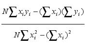
The trend value (C) of each sea level time series, that were used in the ( C x m ) plot was calculated from expressions taken from STANDARD MATHEMATICAL TABLES 17th Edition . Edited by SAMUEL, M.SELBY . The Chemical Rubber Co, 18901, Cranwood,Parkway, Cleveland, Ohio 44128, pages 564, 565:

C = , i = 1,2,………,N (1)

Where x are the sea level heights of the sea level series and y are their corresponding values of instants t of a series with N pairs (x,y).

The correlation (m ) of the N pairs (x,t), was calculated, once the (C) values were known from (1) by using the expression below :

m = , where and, for i = 1,2,…….N (2)

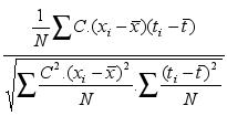
It follows, by putting in evidence ( C/N ) and canceling them in denominator and numerator that:

m = 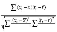, i = 1,2,3…………..N (3)

From which one can see that for each sea level series, the trend value (C) does not appear in expression (3) which was used to determine the correlation (m). Therefore the (m) value does not depend of its corresponding (C) value. Similarly the (C) value does not depend on the (m) value, as the (m) value does not appear in expression (1) used to calculate (C). (C) and (m) are then mutually independent statistical variables.